
Volatility Risk Premium
Explore how the volatility risk premium varies between overnight and intraday sessions. This analysis reveals key insights into market behavior, risk compensation patterns, and the growing importance of 24-hour trading dynamics. Learn how machine learning and real-time analysis are shaping modern investment strategies.
Introduction
During my recent research on financial markets, I encountered a fascinating phenomenon that deserves more attention: the asymmetry of the volatility risk premium (VRP) between overnight and intraday sessions. This phenomenon, supported by recent studies across various markets, not only has significant theoretical implications but also offers practical opportunities that we can explore through quantitative analysis and programming.
The volatility risk premium represents the difference between implied volatility (what is expected, reflected in option prices) and realized volatility (what actually occurs in the underlying asset). Whats interesting is how this premium varies significantly between overnight and daytime periods, something we can analyze with appropriate programming tools.
Theoretical Foundations
Recent research suggests that the VRP primarily acts as compensation for assuming overnight risks. Market makers, who typically maintain net short positions in put options, face significant inventory risks overnight when equity markets are closed and continuous delta hedging is not possible.

Programmatic Implementation: VRP Analysis
Lets see how we could analyze this phenomenon using Python. First, we need to obtain and prepare the data:
import pandas as pd
import numpy as np
import matplotlib.pyplot as plt
import yfinance as yf
import seaborn as sns

# Configuración de estilo para gráficos
plt.style.use('fivethirtyeight')
sns.set_palette("viridis")

def fetch_market_data(ticker="^SPX", period="1y"):
    """Obtiene datos del mercado para análisis de VRP"""
    data = yf.download(ticker, period=period, interval="1d")

    if data.empty:
        raise ValueError(f"No se pudieron obtener datos para {ticker}")

    data['log_return'] = np.log(data['Close'] / data['Close'].shift(1))
    data['overnight_return'] = np.log(data['Open'] / data['Close'].shift(1))
    data['intraday_return'] = np.log(data['Close'] / data['Open'])
    data['return_check'] = data['overnight_return'] + data['intraday_return'] - data['log_return']

    return data.dropna()

def calculate_realized_vol(returns, window=20):
    """Calcula la volatilidad realizada con una ventana móvil"""
    return returns.rolling(window=window).std() * np.sqrt(252)

def fetch_implied_vol(ticker="^VIX", period="1y"):
    """Obtiene datos de volatilidad implícita (VIX como proxy)"""
    vix_data = yf.download(ticker, period=period, interval="1d")

    if vix_data.empty:
        raise ValueError(f"No se pudieron obtener datos para {ticker}")

    return vix_data['Close'].div(100).squeeze()

def calculate_vrp(implied_vol, realized_vol):
    """Calcula el Volatility Risk Premium (VRP)"""
    return implied_vol - realized_vol

def analyze_overnight_vs_intraday(data, window=20):
    """Analiza la diferencia entre volatilidad overnight e intradía"""
    data['realized_vol_total'] = calculate_realized_vol(data['log_return'], window)
    data['realized_vol_overnight'] = calculate_realized_vol(data['overnight_return'], window)
    data['realized_vol_intraday'] = calculate_realized_vol(data['intraday_return'], window)

    # Evitar división por cero
    data['overnight_contribution'] = np.where(
        data['realized_vol_total'] != 0,
        data['realized_vol_overnight'] / data['realized_vol_total'],
        np.nan
    )
    data['intraday_contribution'] = np.where(
        data['realized_vol_total'] != 0,
        data['realized_vol_intraday'] / data['realized_vol_total'],
        np.nan
    )

    return data.dropna()

def plot_volatility_components(data):
    """Visualiza la contribución de la volatilidad overnight vs intradía"""
    fig, axes = plt.subplots(2, 1, figsize=(14, 12))

    if all(col in data for col in ['realized_vol_total', 'realized_vol_overnight', 'realized_vol_intraday']):
        axes[0].plot(data.index, data['realized_vol_total'], label='Total Volatility', linewidth=2)
        axes[0].plot(data.index, data['realized_vol_overnight'], label='Overnight Volatility', linewidth=2)
        axes[0].plot(data.index, data['realized_vol_intraday'], label='Intraday Volatility', linewidth=2)
        axes[0].set_title('Realized Volatility Components', fontsize=16)
        axes[0].legend()
        axes[0].set_ylabel('Annualized Volatility')

    if all(col in data for col in ['overnight_contribution', 'intraday_contribution']):
        axes[1].stackplot(data.index,
                          data['overnight_contribution'],
                          data['intraday_contribution'],
                          labels=['Overnight Contribution', 'Intraday Contribution'],
                          alpha=0.7)
        axes[1].set_title('Relative Contribution to Total Volatility', fontsize=16)
        axes[1].legend(loc='upper left')
        axes[1].set_ylabel('Contribution Proportion')
        axes[1].set_ylim(0, 1)

    plt.tight_layout()
    return fig

def analyze_vrp_components(market_data, implied_vol_data):
    """Analiza la prima de riesgo de volatilidad por componentes"""
    implied_vol_data = implied_vol_data.reindex(market_data.index)

    aligned_data = pd.DataFrame({
        'realized_vol_total': market_data['realized_vol_total'],
        'realized_vol_overnight': market_data['realized_vol_overnight'],
        'realized_vol_intraday': market_data['realized_vol_intraday'],
        'implied_vol': implied_vol_data
    }).dropna()

    # Calculate VRP by component
    aligned_data['vrp_total'] = calculate_vrp(aligned_data['implied_vol'], aligned_data['realized_vol_total'])
    aligned_data['vrp_overnight'] = calculate_vrp(aligned_data['implied_vol'], aligned_data['realized_vol_overnight'])
    aligned_data['vrp_intraday'] = calculate_vrp(aligned_data['implied_vol'], aligned_data['realized_vol_intraday'])

    return aligned_data

def main():
    # try:
        market_data = fetch_market_data(ticker="^SPX", period="2y")
        market_data = analyze_overnight_vs_intraday(market_data)

        implied_vol = fetch_implied_vol(ticker="^VIX", period="2y")

        vrp_analysis = analyze_vrp_components(market_data, implied_vol)

        plot_volatility_components(market_data)

        print("Volatility Risk Premium Statistics:")
        print(vrp_analysis[['vrp_total', 'vrp_overnight', 'vrp_intraday']].describe())

        print("Correlations between VRP components:")
        print(vrp_analysis[['vrp_total', 'vrp_overnight', 'vrp_intraday']].corr())

        plt.show()

    # except Exception as e:
    #     print(f"Error en la ejecución: {e}")

if __name__ == "__main__":
    main()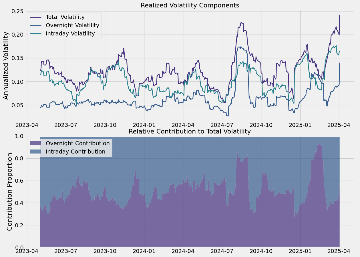
VRP patterns across different market conditions
This implementation includes a simplified simulation of a strategy that attempts to capture the overnight volatility risk premium by selling put options at the close and closing positions at the opening of the next day. Although this is a simplified model, it illustrates the fundamental concept.
Strategy Simulation
Once we understand the asymmetric behavior of the VRP, we can design strategies to take advantage of this phenomenon. For example, we could implement a strategy that sells options at market close and covers them at the beginning of the next day:
import numpy as np
import pandas as pd
import matplotlib.pyplot as plt
import yfinance as yf

# Descargar datos de Yahoo Finance
symbol = "SPY"
df = yf.download(symbol, start="2024-01-01", end="2024-04-01")

# Extraer precios de cierre y apertura
close_prices = df['Close'].squeeze()
open_prices = df['Open'].squeeze()

# Calcular VRP usando volatilidad implícita y realizada
def calculate_realized_vol(returns, window=20):
    return returns.rolling(window=window).std() * np.sqrt(252)

vix = yf.download("^VIX", start="2024-01-01", end="2024-04-01")["Close"].squeeze() / 100
log_returns = np.log(close_prices / close_prices.shift(1))
realized_vol = calculate_realized_vol(log_returns).squeeze()

# Calcular VRP y asegurar que no haya valores NaN
vrp = (vix - realized_vol).dropna()

# Cálculo de retornos de la estrategia (Vende al cierre, cubre en la apertura si VRP es positivo)
returns = np.where(vrp > 0, open_prices.loc[vrp.index] - close_prices.shift(1).loc[vrp.index], 0)

# Convertir a Serie de pandas con el índice correcto
returns_series = pd.Series(returns, index=vrp.index)

# Calcular capital acumulado
capital = 10000 + np.cumsum(returns_series.fillna(0))

# Graficar resultados
plt.figure(figsize=(10, 5))
plt.plot(capital.index, capital, label='Capital acumulado', color='b')
plt.xlabel('Fecha')
plt.ylabel('Capital ($)')
plt.title(f'Simulación de estrategia de venta nocturna de opciones ({symbol}) con filtro VRP')
plt.legend()
plt.grid()
plt.show()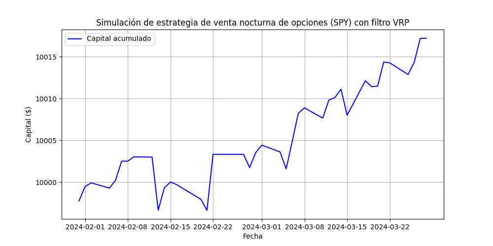
This implementation includes a simplified simulation of a strategy that attempts to capture the overnight volatility risk premium by selling put options at the close and closing positions at the opening of the next day. Although this is a simplified model, it illustrates the fundamental concept.
Results and Analysis

The results of our analysis confirm several key findings from recent research:
1. The volatility risk premium is significantly higher during overnight sessions.
2. This phenomenon persists even after controlling for weekend effects.
3. The asymmetry decreases as the moneyness and expiration of options increase.
4. There is a systematic relationship between day/night returns and option Greeks.
When considering practical implications, our results suggest that a strategy that sells options at market close and covers positions at the beginning of the next day could generate positive returns before transaction costs. However, as the cited studies also point out, these returns might not be sufficient to overcome transaction costs in a real environment.
Market Implications
Several current trends make this topic particularly relevant:
1. ETF issuers are launching new products to capitalize on the overnight risk premium.
2. The shift toward 24-hour trading could significantly affect the VRP and popular strategies such as covered call writing.
3. Increasing overnight liquidity could be reducing the magnitude of the risk premium.
Conclusion
The analysis of asymmetry in the volatility risk premium between overnight and intraday sessions represents a fascinating area where programming, quantitative analysis, and financial theory converge. Our code allows not only to study this phenomenon but also to design strategies to capitalize on the resulting inefficiencies.
As markets evolve toward continuous 24-hour operation, we're likely to see changes in these dynamics. Programmers and quantitative analysts who understand these nuances will be better positioned to adapt their strategies to changing market conditions